Team A (Factor Analysis) - Ankit Jaiswal (Mktg)

Factor analysis is a statistical method used to describe variability among observed, correlated variables in terms of a potentially lower number of unobserved variables called factors. This analysis is based on dependent variables and independent variables.

For example, Sales of any product is generally dependent on factors like customer satisfaction, marketing speed, product, etc. So in this case, factors like customers satisfaction, marketing speed, product are independent variables, and sales, on the other hand, is dependent variable.

In factor analysis, we find whether the independent variables are related to each other in some or the way. We do not drop the variables, but instead we combine them and try to remove the correlation between them. The independent variables are combined together on the basis of the correlation, and the ones which are more correlated are combined and a cluster is formed. The information gained about the interdependencies between observed variables can be used later to reduce the set of variables in a dataset.

Reasons to perform Factor Analysis

• To reduce the variables and remove the correlation between them, so that we get a better picture of the scenario.
• To see and find the common underlying theme and label them.

An ideal scenario to perform factor analysis is when there is large number of variables and all of them are correlated with each other. In this analysis, only scale numbers are considered.

To conduct a Factor Analysis, start from the “Analyze” menu.  This procedure is intended to reduce the complexity in a set of data, so we choose “Data Reduction” from the menu.  And the choice in this category is “Factor,” for factor analysis.

After we click on factor, the following dialog box appears

From this dialogue box, string variables like manufacturer name, model name, etc are not selected, only the scale numbers are selected.

From the Descriptive, we check the Initial solution option.

From the Extraction, check Scree plot, and check eigenvalue to be greater than 1.

From the Rotation, check Varimax option.

Now after the output file we get, we see the Communalities output, which is as under:

In the above table, the Initial column shows that the variance for the different variables is 1, and the Extraction column shows that the amount of extraction that is possible from that particular variable. The thumb rule is that if the extraction value for any variable is below 0.5, then we drop it. In the above box, sales have let extraction, i.e. 0.403. So if we remove the sales as one of the variable, we see that the extraction rises to 80%-90%, as seen under

After this, we copy the data of one variable, suppose price to excel sheet. And find the average of the entire data of the price of the cars, and find out the variance from the average. We also find out the standard deviation of the data, which helps us to find the Z score (Variation/Std Dev). The properties of the Z score is that it retains the distribution of the data, and, their mean = 0, and Std. Dev = 1.

Components are made of some amount of variance of all types. In the table ‘Total Variance’, Total resembles Variance.

The above table shows that the first two components are not correlated and account for almost 82% out of the total 100%. Rest 18% is covered by the remaining 8 components. Varimax method makes the variance of the different components appear in the descending order with variables having more % t the top. The other columns in the table shows that we move forward with the components 1 and 2 as they are not correlated.

Then we come to the Component matrix, it shows the relation of the component with the variable.

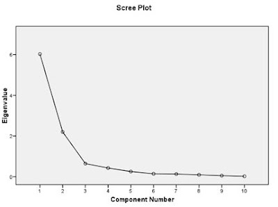
Scree plot helps in choosing the number of components out of the total number of variables. In this case, we choose component 1 & 2 as after that its almost constant, as can be seen under:

Rotation Component Matrix

This is the critical element of the Factor analysis. Rotation tries to equalise the variance, making sure that the cumulative variance remains the same.

We do the rotation so that the dominant variable can be identified & also find out what it is made of. The rule is whichever variable has higher value in component 1 and lesser value in component 2 is selected. The difference between the two should be at least 0.30. the rotation matrix looks as under

In the above figure we can see that, in component 1, variables like wheelbase, width, length have greater values and all of these shows us the specifications of the car, so we label it as SPECS. In component 2, variables like 4-year resale value, price, horsepower have greater values so we label them as PRICE as all specifies the price except horsepower. This shows that there is a possibility of 3^rd component.